Numbers
Thursday at the library
It’s Thursday afternoon and the von der Surwitz siblings meet in their reserved study room at the main university library to go over Wednesday’s lecture and examples. After Wednesday’s class, they’re glad they and the other ItCS participants had met with Professor Chandra at the Novalis Tech Open House two weeks prior to the start of school and had gotten a heads-up on what was ahead, including her repository. As a result they all had gone down the minimal prerequisite rabbit holes and were more or less ready.
Ursula von der Surwitz has plugged in her laptop to the big monitor and is scrolling through Professor Chandra’s first substantive lecture on Wednesday of the first week of classes1 This is also on her GitHub repository. .
⌜…
For most of us our first experience with the abstraction power of
numbers begins when our parents teach us to hold up three fingers to
show everyone we’re three years old. And so we were introduced to the
idea of seeing an abstract numerical magnitude such as the number
three as a mapping or connection of three fingers to three years of
life.
Then at some point we learn what mathematician Eugenia Cheng2 See her popular layman’s book How To Bake \(\pi\;\). One interesting aspect of this book is her treatment of category theory, which is a superset of type theory, much of which is baked into Haskell. calls the “counting poem,” i.e., we learn how to count from one to ten, usually on our fingers. And about this time we learn to negotiate numerically, like when we said, I’ll give so many of these if you give me so many of that. But then begins formal school math, and each year math becomes progressively less interesting, less popular — to the point of being a hated subject. This in my opinion is due to the curriculum being based on conditioned learning, the when you see this, do this method … unfortunately.
But if you major in math in college you eventually start to see in the later years3 In many places in the world the typical American college Freshman-Sophomore math sequence of calculus, diff-eqs, and linear algebra is completed at the college-prep level. For example, Germany and Switzerland have college freshmen starting with Analysis. — after the four Freshman and Sophomore semesters of calculus, differential equations, and linear algebra — what is commonly called “higher math.” And these upper-semester math courses can be a complete reboot of math, weeding out vague, ad hoc, parochial4 parochial: … very limited or narrow in scope or outlook; provincial… notions, replacing them with a rigorous, theoretical, formalistic, foundational understanding of math. As mathematician Joe Fields says, this is when you stop being a “see this, do this” calculator and become a prover, i.e., a deeper thinker about math.
Set theory is a big part of this formalism5 Make sure you’re attacking the LibreTexts series, e.g., one of the first three rabbit holes in the math section. . Set theory is an exacting, don’t-take-stuff-for-granted world, which turns out to be good for the computer world as well since computer circuits don’t attend human grade school, don’t learn poems, and don’t have fingers6 If machines were capable of conditioned learning, your car should be able to self-drive certain oft-travelled routes, e.g., from your home to the grocery store. . Again, if you want a computer to understand something, you have to spell it out in very precise and exacting ways. That is to say, you’re always facing logical entailment (LE) with computers. So how then does a computer understand numbers? And isn’t a computer doing numbers the same way a clock does time? Think about it. Does a ticking clock that you have to wind up have any real concept of time? No, it doesn’t.
One fascinating twist of mathematical history is how, on the whole, the Greeks seemed to favor geometry over numbers. Their mastery of geometry really got going with Euclid’s Elements ca. 300 BC, which starts with just a point and a line and from there builds up expansive theorems about complex geometric shapes, i.e., no numbers7 It was a long-revered feat of logical minimalism that all two-dimensional shapes in Elements could be produced with just a compass and a straightedge. Follow the Wikipedia link and note the animation of the construction of a hexagon. It wasn’t until the development of calculus and infinitesimal methods in the Renaissance that this compass-and-stick purity was set aside. . Even when Euclid’s geometry worked with the concepts of length and angles, no numbers were employed8 Later we’ll explore how Descartes united algebra and geometry. . And as the physicist Julian Barbour said, A triangle is known for its shape not its size.
This week we’ll talk about numbers in a fairly theoretical but not
really difficult manner. Along with the math, we’ll do some work with
Haskell that you should be ready for9
Make sure you’re getting along with the Haskell rabbit hole materials — at
the very least worked through half of LYAHFFG.
.
…⌟
𝔘𝔯𝔰𝔲𝔩𝔞: So like
Professor Chandra said yesterday, we need to see things in terms of
set theory from here on out.
[murmurs of agreement]
𝔘𝔴𝔢: And like she said,
with set theory we can properly define relations and function. All of
which sounds rather ominous. Like everything we thought we knew was
about to go away.
[more agreement murmurs]
𝔘𝔯𝔰𝔲𝔩𝔞: [continuing] So
here’s her breakdown of what she called number classification or
taxonomy. [scrolling…]
⌜…
- \(\mathbb{N}\;\): the natural counting numbers, often starting with \(0\;\); otherwise, with \(1\;\).
- \(\mathbb{Z}\;\): whole number integers — just like \(\mathbb{N}\;\) but with the positive numbers duplicated as negative numbers, along with \(0\;\) between them.
- \(\mathbb{Q}\;\): the rational numbers — composed as \(\frac{a}{b}\;\) where \(a\) and \(b\) are integers and \(b\) cannot be \(0\;\) — although this is really too simple and we’ll be expanding on it later.
- \(\mathbb{R}\;\): the real numbers are the limit of a convergent sequence of rational numbers… Really? Yes, but this is a higher math sort of definition. Suffice it to say for now reals are the rational numbers (including recurring decimals) along with ir-rational numbers (non-recurring decimals), e.g., the square root of \(2\;\). In other words, numbers that are expressed with decimals10 Two questions: Are repeating decimal numbers also rational? If yes, then why can’t rational numbers represent all numbers? That is, why do we need real and complex numbers? Programming challenge: Write a function that takes a real decimal number and figures out its fraction, e.g. \(3.14\) is \(157/50\:\). Does Haskell have a built-in way to do this? Hint: Check out Convert decimal number to rational. Maybe compare with how Julia and Racket do it. . Lots more to come…
- \(\mathbb{C}\;\): the complex numbers are of the form \(a + bi\;\) where \(a\) and \(b\) are real numbers and \(i\) is the square root of \(-1\;\). Again, lots more later.
…⌟
𝔘𝔴𝔢: Right. We’re not
supposed to worry about this too much yet; we’ll go into it more
later. Just realize that we’re talking about the set of natural
numbers, the set of real numbers, et cetera.
[murmurs of agreement]
𝔘𝔱𝔢: Their traits and
properties, as she said. And the fact that each number “species” is a
subset of the next one up [writing on the whiteboard]
𝔘𝔱𝔢: [continuing] One
is contained by the other.
𝔘𝔴𝔢: [paging through
his written notes] Then she once more drove home the point that set
theory is important [quoting]
⌜…
Set theory is the basic foundation of math, and is fundamental to the
discrete math of computer science. But there’s a new kid is on the
block, namely, category theory, which is even more foundational than
set theory. With Haskell we’ll encounter some of the rudiments of
category theory now and then.
…⌟
𝔘𝔴𝔢: Anybody know what
that means?
𝔘𝔯𝔰𝔲𝔩𝔞: We all watched
the video? [clicking on this YouTube link] Did you all watch it?
𝔘𝔱𝔢: Ahhh, yes, but I
can tell I’m a long way from really getting it, or why it’s such a big
deal.
𝔘𝔴𝔢: So we see a bunch
of stuff we supposedly already know being repackaged in a way that
uncovers how we really only had a superficial understanding of the
concepts.
[laughter]
𝔘𝔯𝔰𝔲𝔩𝔞: I watched it,
but it’ll take some time to sink in because [nodding to Uwe] on one
level I guess I understood, but I don’t think I caught what the whole
point was11
Professor Chandra connected this to Haskell by mentioning
Haskell’s “point-free” programming … but didn’t elaborate.
. I suppose that’s coming as well.
𝔘𝔱𝔢: But wasn’t it a
bit ominous the way she said this is higher math — if not grad
school stuff? But we’re not supposed to be intimidated! No! At least
not yet.
[nods and laughter]
𝔘𝔴𝔢: Like they’ve been
saying, we’re Versuchskaninchen.
[laughter]
𝔘𝔱𝔢: Guinea pigs. No,
but I’m getting the impression this could be a great course.
[nods]
Numbers in Haskell
𝔘𝔯𝔰𝔲𝔩𝔞: [scrolling] So
we then come to Haskell’s version of the numbers.
[all study the screen]
𝔘𝔱𝔢: Which is supposed
to be close to the whole mathematical taxonomy.
⌜…
Int: limited-precision integers in at least the range \([-2^{29} , 2^{29})\;\).Integer: arbitrary-precision integers (read lots of integers, lots more thanInt).Rational: arbitrary-precision rational numbers.Float: single-precision floating-point numbers.Double: double-precision floating-point numbersComplex: complex numbers as defined inData.Complex.
…⌟
𝔘𝔯𝔰𝔲𝔩𝔞: And she tells
us not to worry about what precision and floating-point mean for
the time being.
𝔘𝔱𝔢: Right, because
they’re part of how the electrical logic circuits do numbers. The
whole “logical entailment” of doing numbers on an electric machine
thing.
[murmurs of agreement]
𝔘𝔴𝔢: And we’re not to
worry about natural numbers yet. We’ll do those separate.
[murmurs of agreement]
The qualities of quantity
𝔘𝔯𝔰𝔲𝔩𝔞: [scrolling] So here’s more.
⌜…
A number is a concept, first and foremost a symbol related to
quantity and magnitude. And as such a number has great powers of
abstraction. Numbers may be applied in the abstraction exercises of
counting or enumerating, as well as measuring things12
But then measuring must be “quantified” by counting unit-wise
what was measured; hence, everything comes back to counting. This will
come up when we explore real numbers versus rational numbers.
.
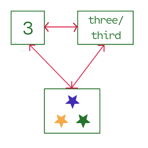 The concept, the embodiment of three and "three-ness"
Consider these qualities of quantities
- cardinality, or how many?
- ordinality, or what order?
- enumeration, or, generally, how do we count out things?
As we’ve said, when we bring the computer into this quantification
game, we cannot assume these basic qualities as given13
Inside your head you automatically know how many and in what
order the numbers \(1\) through \(10\) are. However, a computer must be
taught such basic quantitative qualities.
.
…⌟
𝔘𝔯𝔰𝔲𝔩𝔞: [continuing]
Any thoughts, questions?
[all study the screen]
𝔘𝔱𝔢: Let’s go on.
Cardinality
⌜…
In everyday language cardinal numbers are simply the counting numbers,
\(\mathbb{N}\;\), either as words or numerical symbols. In set theory,
however, cardinality has a different meaning, i.e., the number the
objects in a set. So if we consider the box of stars in the diagram
above to be a set of stars, then the cardinality of this set is \(3\)
since there are three stars14
We indicate the set’s cardinality by surrounding the symbol for
a set with pipes ( | ), e.g., \(|S_{stars}|\;\). This is not the same
as absolute value, although they might be cousins.
But why are we being so “conceptual” about the simple idea of amount, and why must we give it a fancy name? Again, math likes to formalize things, nail things down. Starting with exactness and precision we can then build very complex and logically-based math15 Have a look at this Wikipedia discussion of cardinality. Later we will look into cardinal numbers, which is a deeper dive into set theory. . Now, if two sets have the same cardinality, is this somehow significant? Above, we see that both the set of natural numbers and the set of integers have infinity as their cardinality. Are, therefore, \(\mathbb{N}\) and \(\mathbb{Z}\) the same “size?”
The bijection principle states that two sets have the same size if and only if there is a bijection (injective and surjective together) between them16 We’ll look at injective, surjective, and bijective when we delve into functions from a set theory perspective. Also, mathematical logic will introduce us to if and only if. .
Which means \(|\,S_{stars} \,|\;\) and \(|\,\{a, b, c\}\,|\;\) can be matched
up one-to-one, thus, they must have the same cardinality. But again,
what about sets of things that supposedly have an infinite size? How
do we “count,” or “pair up” infinite sets17
To excite your curiosity, isn’t \(\infty + 1\) still just \(\infty\;\)? The
Greeks contemplated this and concluded that infinity has the power to
consume, destroy individual numbers. It wasn’t until the German
mathematician Georg Cantor came along in the late nineteenth century
that we learned to wrangle infinity.
? Surprisingly, there
are different kinds of infinity — which necessitates this exactness
and preciseness. More about cardinality theory later.
…⌟
𝔘𝔴𝔢: So basically,
cardinality is a formalism from set theory about amount and
magnatude. Fair enough.
𝔘𝔯𝔰𝔲𝔩𝔞: What about this
section? [scrolling]
Haskell and cardinality
⌜…
The first thing to know about Haskell and set theory is, yes, we can
do real set theory with Haskell’s Data.Set package. But as beginners
learning the ropes we will start with a simpler representation of sets
through Haskell’s basic list data structure. Realize, however, that
a list is not a set; they are two different beasts, and we’ll have to
account for that. For one, a set may have duplicates, whereas a list
holds a definite sequence of things, i.e., every element of the list
is unique, even if some elements are repeated18
So it’s not really a “grocery list,” it’s a “grocery set”
since \(\{eggs,sugar,coffee,eggs\}\;\;\;\) is invariably interpreted as
just \(\{eggs,sugar,coffee\}\;\;\), right? Or would you go ahead and get
eggs twice? Can you come up with another real-world example where a
set of things doesn’t care about order or duplicates?
. So the set
\(\{1,2,1\}\;\) is the same as \(\{1,2\}\;\) is the same as \(\{2,1,1\}\;\)
because sets don’t mind duplicates, nor do they worry about
order19
Why is this? There is a LE to the definition
of a set union, namely, \(A \cup B = \{x \;\;|\;\; x \in A \;\;\;or\;\;\; x \in
B \}\quad\). Consider the sets \(A = \{1,2,3\}\;\), \(B = \{2,3,4\}\;\),
and \(C = \{3,4,5\}\;\). If you draw out Their union \(A \cup B \cup C = \{x
\;|\; x \in A \;\;\text{or}\;\;x \in B\;\; \text{or}\;\;x \in C \}\quad\;\;\) as
a Venn diagram, you’ll see how duplicates get left out.
. But the lists [1,2,1], [1,2], and [2,1,1] are in
fact all different lists. Initially, we’ll practice set theory with
lists and build alternate set theory code based on lists. Then when we
understand “squirrel math” a little more, i.e., how to work with the
data structures known as trees, we’ll do proper set theory with
Haskell’s set theory module, Data.Set20
Take a look at this Hackage page. It has an intro to Haskell’s
sets. Get in the habit of perusing Hackage whenever you’re using a
Haskell function or data type you don’t quite understand. Sometimes
you’ll have to just dive into the code, but sometimes there are
excellent intro docs like this. And yet there are also set operations
in Data.List. Perhaps look into these two options.
. For the immediate
future we’ll consider a list to be a beginner’s substitute for a
set. And so a simple “how many” function on a list standing in for a
set is length. The code length [1,2,3,4,5] \(\implies\) 5. Again,
more to come. Watch this space21
Meanwhile, here’s a brain-teaser that goes to the heart of
this set-list issue — especially in Haskell, Why are set union and
intersection commutative and associative due to their lack of order?
. …⌟
𝔘𝔴𝔢: So, bottom line,
we’re not going to have real sets with Haskell right away, just a sort
of Ersatz sets with lists. Are we all sort of familiar with Haskell
lists from the Learn You…?
[murmurs of affirmation as Ursula clicks on a tab showing LYAHFGG’s
section on lists]
𝔘𝔱𝔢: So what about
finding another example of sets having duplicates and being in
different order? [looks back and forth]
𝔘𝔯𝔰𝔲𝔩𝔞: Well, here’s
mine [scrolling to her personal annotation of the professors notes and
reading aloud]
⌜…
A “set” of students in a class pass around a sign-in sheet each day on
which they sign their name. Some days the names are in one order,
other days another order, depending on how it was passed around the
room. And sometimes a student accidentally signs twice. But it’s still
the same set of students, order and duplicate sign-ins
notwithstanding.
…⌟
𝔘𝔴𝔢: Oooh,
notwithstanding! You’re getting fancy with your English.
[laughter]
𝔘𝔯𝔰𝔲𝔩𝔞: Hey, no
brain-shaming!
[laughter]
𝔘𝔴𝔢: [continuing] No,
really, that’s a great example because it brings out the difference
between the actual set and how it’s being — represented.
𝔘𝔱𝔢: So do we all
understand her side note about set unions?
𝔘𝔴𝔢: I drew some Venn
diagrams [pulls out a hand drawing and places it on the table] and,
yes, you can see how all the overlaps are telling us not to worry
about the duplicates of the individual sets making up the union.
𝔘𝔱𝔢: Right, and it’s
curious how when you just look at the set notations, you don’t
necessarily see that. At least I don’t. I mean [writing on the board]
\(A \cup B \cup C = \{x \;|\; x \in A \;\;\text{or}\;\;x \in B\;\; \text{or}\;\;x
\in C \}\quad\;\;\) doesn’t necessarily tell you it doesn’t want
duplicates.
𝔘𝔴𝔢: By the way, don’t
forget union and intersection are binary, right?
[nods of agreement]
𝔘𝔱𝔢: All right then,
[correcting her formula] \(A \cup B = \{x \;|\; x \in A \;\;\text{or}\;\;x \in
B\;\}\;\;\;\;\). Satisfied?
[Ursula giggles]
𝔘𝔴𝔢: All right, unless
you have the word or to mean that we don’t keep picking up the same
element from the different sets. But the inclusive or of set union
means it can be from one or the other — or from both of
them. So I definitely see your point, the set notation doesn’t tell
us not to include duplicates — without some exclusive sort of
inclusive or. Only the Venn diagram really shows us this. I mean,
the whole point of this is to think about whether the definition of
set union rules out duplicates, doesn’t worry about order, and has
commutativity. I don’t see that
[murmurs of agreement]
𝔘𝔱𝔢: So in the rabbit
hole on logic, we had the truth tables, right? So they talked about
logical or, which they also called disjunction. And then they had
a truth table for or which showed how the only time something wasn’t
true was when both of the statements were false.
𝔘𝔴𝔢: Basically, it’s
the same operations with both sets and logic.
𝔘𝔯𝔰𝔲𝔩𝔞: More later.
[murmurs of agreement]
𝔘𝔯𝔰𝔲𝔩𝔞: All right, so
what about this brain teaser?
𝔘𝔱𝔢: Right. [getting up
and writing on the board]
𝔘𝔱𝔢: [continuing] The
first thing we have to know is what are union and intersection in the
world of lists? I figured out that putting lists together come in two
forms, the cons operation, and the concatenation operator.
𝔘𝔯𝔰𝔲𝔩𝔞: Right. Like
this. [creating a source block]
1 : []
[1]
𝔘𝔯𝔰𝔲𝔩𝔞: [continuing]
for cons and then this for concatenation
[1] ++ [2]
[1,2]
𝔘𝔴𝔢: You showed me that
stackoverflow post where they created a union function for
lists. But then one commentor noted how no, these list versions of
union didn’t allow for commutativity and all.
𝔘𝔯𝔰𝔲𝔩𝔞: Exactly. Only
the Data.Set, the true set theory package did.
[silence while digesting the ideas]
𝔘𝔱𝔢: Yeah, right, I
looked through it, but I consider myself just a beginner with Haskell,
but it seemed to be talking mainly about how you eliminate
duplicates.
𝔘𝔴𝔢: But what about
that “equational reasoning”? One of you guys went into that, didn’t
you?
[Ursula and Ute trade glances]
𝔘𝔱𝔢: Well, I looked it
up on Wikipedia and was redirected to an article that was actually
called Universal algebra [Ursula brings up the article on the
monitor], and in the Basic idea section
𝔘𝔴𝔢: Once again, on
that fateful day when we sat down and talked with Professor Chandra
she told us to not fear the rabbit hole!
[laughter]
𝔘𝔱𝔢: And to expect a
whole new way of seeing math.
𝔘𝔴𝔢: Right, that didn’t
present itself serially, one thing after another. No, we’re taking
this on in parallel.
[murmurs of agreement]
𝔘𝔱𝔢: I did email
Professor Chandra, and she said the Universal algebra page was not
very specific for what Haskell meant by equational reasoning — and
she gave me another link, which we can look at — but that it
contained a lot of good stuff, and we should try to get the gist of
it.
[rueful murmurs]
𝔘𝔱𝔢: [continuing,
reading from her laptop]
⌜…
An algebraic structure consists of a nonempty set \(A\) (called the
underlying set, carrier set or domain), a collection of
operations on \(A\) (typically binary operations such as addition and
multiplication), and a finite set of identities, known as axioms, that
these operations must satisfy.
…⌟
𝔘𝔯𝔰𝔲𝔩𝔞: [bringing the page up on the monitor] Here it is.
import Data.Set (Set, lookupMin, lookupMax)
import qualified Data.Set as Set
Set.union (Set.fromList [1, 3, 5, 7]) (Set.fromList [0, 2, 4, 6])
fromList [0,1,2,3,4,5,6,7]
Set.union (Set.fromList [0, 2, 4, 6]) (Set.fromList [1, 3, 5, 7])
fromList [0,1,2,3,4,5,6,7]
Set.empty
fromList []
Set.union (Set.fromList [1,2,3]) (Set.empty)
fromList [1,2,3]
Set.intersection (Set.fromList [1,2,3]) (Set.empty)
fromList []
import Data.Ratio
𝔘𝔯𝔰𝔲𝔩𝔞: Let’s leave it for now. So moving on [scrolling].
Ordinality
⌜…
In everyday language the concept of order is conveyed when we say
first, second, third, fourth, etc22
See this brief discussion.
. And we’re done, right? But
again, as seen from set theory — as well as from the computer world
— (re-)establishing order is important and cannot always be taken
for granted. In fact, a great deal of investigation surrounds
ordinality.
The counting numbers, the set \(\mathbb{N}\;\), would seem to have order built in. For example, everybody knows that \(3\) comes after \(2\;\) etc., they’re in ascending order based on the incrementally greater amounts they represent. And neither does the set \(\mathbb{N}\;\) have repeats. Also, if we create a geometric visual for \(\mathbb{N}\;\), that is to say, we draw a line and mark places on the line for each number, we can subdivide the line into intervals23 Typically, real numbers are represented geometrically by a “number line” whereby interval notation allows for sections of this line to be considered, e.g., closed interval \([\,a,b\,]\;\), open interval \((a,b)\:\), and more exotics like an open ray \((-\infty, a)\:\). and order is related to inequalities.
But order, and all it’s implications, is not always a given in real life. What if we wrote the numbers from one to ten on small squares of paper, put them in a box, and then shook them out on the floor in a straight line? Would they be in order? Chances are, no. And what about sets of things that aren’t inherently numerical, such as colors?
So if we don’t have things in proper order—which is often the case in the real world—we have to put things in order ourselves. And that means we will need to sort a set of unsorted elements into some order. Sorting, in fact, is one of the more basic tasks computers do in the everyday world24 We will eventually investigate how costly in computer time and resources an operation like sorting is. Stay tuned. .
But to sort we need to compare things. Obviously, ten whole numbers written clearly on ten squares of paper can be easily sorted by hand25 A jigsaw puzzle can be seen as a sorting game based on shape, color, and patterns of the pieces. . But what if we had thousands of squares of paper, each with a unique number? Then we’d have a long task ahead of us. But no matter how big or small the task, we would compare two numbers at a time and then make a judgement based on whether one number was
- greater than
- equal to
- less than
the other number, then rearranging as needed.
…⌟
Ordinality in Haskell
Haskell is a typed language with a feature called type classes26 For a quick introduction with examples go here in LYAHFGG. . A Haskell type class encompasses traits, patterns, concepts, or what we might call a certain “-ness” that can be imparted to data types. In Haskell, for example, numbers and the characters of the alphabet can be directly compared for “equal-ness,” and when we test at the ghci REPL prompt, this seems to be built-in
((5 == 3) || ('a' == 'a')) || ('b' == 'B')
True
Mindful of LE, we see that Haskell’s Eq class
housing this equal-ness must have some sort of behind-the-scenes
mechanism that allows us to take two things, analyze them, then return
a decision, true or false (yes they are equal, no they’re not equal),
on whether two said things were equal or not — all of this just for
doing some typing, e.g., 5 == 3 into the REPL.
Something else to consider is how some things don’t necessarily have
the concept of equal or not equal straight out of the box. What if we
created a data type for colors and we wanted to compare the individual
color values for equal-ness? Intuitively, we might say red, yellow,
and blue are equal since they are all primary colors; likewise,
orange, green, and violet are equal because they’re the secondary
colors. But what if we just say each color is equal to itself and not
equal to any of the others? … So how would we establish equal-ness
for colors? If we want to type Green == Blue into the REPL it’s up
to us to have created some sort of equal-ness and told Haskell about
it.
Data types that need to establish equal-ness for themselves can apply
to the Haskell Eq type class for membership. Type class membership
is registered with an instance statement. To see all the data types
that have an instance registered with Eq we can use :info
(abbreviated :i) at the REPL27
Go ahead and check out the hackage.haskell.org entry for Eq
here. Note the properties (==) should follow: reflexivity, symmetry,
transitivity, extentionality, and negation. We’ll dive into what this
all means when we look closer into the higher algebra of sets and
functions. Note all the built-in, “batteries-included” Eq instances
for the various types. Some are rather exotic.
:i Eq
type Eq :: * -> Constraint
class Eq a where
  (==) :: a -> a -> Bool
  (/=) :: a -> a -> Bool
  {-# MINIMAL (==) | (/=) #-}
  	-- Defined in ‘ghc-prim-0.7.0:GHC.Classes’
...
instance Eq Int -- Defined in ‘ghc-prim-0.7.0:GHC.Classes’
instance Eq Float -- Defined in ‘ghc-prim-0.7.0:GHC.Classes’
instance Eq Double -- Defined in ‘ghc-prim-0.7.0:GHC.Classes’
instance Eq Char -- Defined in ‘ghc-prim-0.7.0:GHC.Classes’
instance Eq Bool -- Defined in ‘ghc-prim-0.7.0:GHC.Classes’
...
which gives us a long list (abbreviated above) of data types that have
equal-ness defined28
Quick LE question: Can functions be compared for equal-ness?
Here’s a direct quote from a prominent combinatorics text: When two
formulas enumerate the same set, then they must be equal. But not so
fast in the computer world. To say f x == g x Haskell isn’t
logically set up to actually prove (demonstrate) and accept that f
and g always give the same results given the same x input. We
would literally have to test every possible x, which is not
possible. Still, we’ll examine this idea a bit closer soon. It’s a
real big deal in numerical math.
. Notice the two “prescribed” methods (functions)
(==) and (/=). These functions are the mechanism used by Eq to
establish equal-ness. They must be custom defined in each instance
declaration in order for a data type to have its own established
equal-ness29
Note {-# MINIMAL (==) | (/=) #-} which is a directive
meaning we may choose to define either (==) or (note the or
pipe | ) (/=), i.e., we don’t actually have to define both because
by defining one, the other will be automatically generated. Neat.
. And so if you create a new type, you, the
programmer, must come up with your own version of these two functions,
(==) and (/=) to establish the trait, the property of equal-ness
for that new data type. As LYAHFGG notes, the type signature for the
equal-ness function (==) is30
:t is short for :type.
:t (==)
(==) :: Eq a => a -> a -> Bool
which indicates (==) takes two inputs of some type a and returns a
Bool type, i.e., either True or False. Good, we saw how that
works with our examples above. But there’s another wrinkle to this
story. So if (==) is a function that takes two objects of type a,
e.g., two integers, real numbers, characters, booleans, etc., how can
we use this same symbol (==) in so many different contexts? Looking
above, how did Haskell know to use integer equal-ness rules (defined
by instance Eq Int) when comparing integers, and then letter
equal-ness rules (defined by instance Eq Char) when comparing
letters? This feat is what we call ad hoc polymorphism31
ad hoc, from Latin to this, is something put together on
the fly for one narrow, pressing, or special purpose. polymorphic,
from Greek polus much, many, and morphism, having the shape, form,
or structure, i.e., having many shapes.
, which
allows just a single function symbol, e.g., (==), to be used
(overloaded) in many different contexts. And so Haskell figures out
behind the scenes which instance to apply. Neat.
Let’s take a closer look at a color type by defining our own32
As LYAHFGG says, Read and Show are also type classes to
which you may register your data type. Here we’ve used the deriving
keyword to let Haskell figure it out, i.e., we’re not defining
Read and Show ourselves; rather, we’re telling Haskell to
auto-generate and register these instances for us.
, 33
We’ll go into more detail about declaring our own data types
as we progress. But for now we’ll say Color is a sum type, as
opposed to a product type. Sum types are patterned after the
addition principle which we’ll also go into later. Note, the pipes
\(\;|\;\) between the colors can be understood as logical or—as in
we must choose one or the other of the colors.
data Color = Red | Yellow | Blue | Green deriving (Show,Read)
Obviously, the colors red, yellow, blue, and green have no intrinsic
numerical properties by which to compare one with the other. However,
Haskell’s type class system still allows us to create some manner of
equal-ness for it. And so we write this version of an instance of
Eq for Color
instance Eq Color where
  Red == Red = True      -- could also be (==) Red Red = True
  Yellow == Yellow = True
  Blue == Blue = True
  Green == Green = True
  _ == _ = False         -- at this point must be false
And so we’ve hand-coded our own equal-ness for Color by spelling out
how (==) works for Color. This literally tells Haskell what
Color equal-ness should be by customizing how the function (==)
should work. Let’s have another look at the type signature for (==)
:t (==)
(==) :: Eq a => a -> a -> Bool
As LYAHFGG notes, the Eq a part is known as a class
constraint. This means whatever a might be, it must have an
equal-ness instance already registered for it — which we do —
otherwise, Haskell won’t know how to compare two things of a for
equal-ness34
For our Color we’ve created our own equal-ness, although in
this example we could have let Haskell figure it out, i.e., ...|
Green deriving (Eq) would have done the same thing. This was an easy
one. Haskell can’t always figure out the less obvious cases.
. …and this is an example of parametric
polymorphism where the parameter (aka type variable) a can be
any data type. In Haskell, smaller-case letters such as a, b, c,
etc., are generic parameter names and can indicate any data type. In
(==) :: Eq a => a -> a -> Bool we see that two inputs of the same
type a are fed to (==), which produces a Bool output. Another
example would be myFunc :: a -> b -> a. Here the type signature says
the inputs don’t have to be of the same type (although they could be),
but no matter what type the parameter b is, the output will be of
type a. Testing our colors
(Red == Red) && (Red /= Green)
True
Good, it’s working and we now can compare Color values for
equal-ness, but how do we order colors? No matter how we establish
one color before the other, it might seem arbitrary, but we can do it
if we want. For basic order-ness Haskell has the type class Ord to
which types can register
:i Ord
type Ord :: * -> Constraint
class Eq a => Ord a where
  compare :: a -> a -> Ordering
  (<) :: a -> a -> Bool
  (<=) :: a -> a -> Bool
  (>) :: a -> a -> Bool
  (>=) :: a -> a -> Bool
  max :: a -> a -> a
  min :: a -> a -> a
  {-# MINIMAL compare | (<=) #-}
  	-- Defined in ‘ghc-prim-0.9.1:GHC.Classes’
instance [safe] Ord Color -- Defined at src/numbers1.hs:16:10
instance [safe] Ord Color2 -- Defined at src/numbers1.hs:28:70
instance Ord Integer -- Defined in ‘GHC.Num.Integer’
instance Ord () -- Defined in ‘ghc-prim-0.9.1:GHC.Classes’
instance (Ord a, Ord b) => Ord (a, b)
  -- Defined in ‘ghc-prim-0.9.1:GHC.Classes’
instance (Ord a, Ord b, Ord c) => Ord (a, b, c)
  -- Defined in ‘ghc-prim-0.9.1:GHC.Classes’
instance (Ord a, Ord b, Ord c, Ord d) => Ord (a, b, c, d)
  -- Defined in ‘ghc-prim-0.9.1:GHC.Classes’
instance (Ord a, Ord b, Ord c, Ord d, Ord e) => Ord (a, b, c, d, e)
  -- Defined in ‘ghc-prim-0.9.1:GHC.Classes’
instance (Ord a, Ord b, Ord c, Ord d, Ord e, Ord f) =>
         Ord (a, b, c, d, e, f)
  -- Defined in ‘ghc-prim-0.9.1:GHC.Classes’
instance (Ord a, Ord b, Ord c, Ord d, Ord e, Ord f, Ord g) =>
         Ord (a, b, c, d, e, f, g)
  -- Defined in ‘ghc-prim-0.9.1:GHC.Classes’
instance (Ord a, Ord b, Ord c, Ord d, Ord e, Ord f, Ord g,
          Ord h) =>
         Ord (a, b, c, d, e, f, g, h)
  -- Defined in ‘ghc-prim-0.9.1:GHC.Classes’
instance (Ord a, Ord b, Ord c, Ord d, Ord e, Ord f, Ord g, Ord h,
          Ord i) =>
         Ord (a, b, c, d, e, f, g, h, i)
  -- Defined in ‘ghc-prim-0.9.1:GHC.Classes’
instance (Ord a, Ord b, Ord c, Ord d, Ord e, Ord f, Ord g, Ord h,
          Ord i, Ord j) =>
         Ord (a, b, c, d, e, f, g, h, i, j)
  -- Defined in ‘ghc-prim-0.9.1:GHC.Classes’
instance (Ord a, Ord b, Ord c, Ord d, Ord e, Ord f, Ord g, Ord h,
          Ord i, Ord j, Ord k) =>
         Ord (a, b, c, d, e, f, g, h, i, j, k)
  -- Defined in ‘ghc-prim-0.9.1:GHC.Classes’
instance (Ord a, Ord b, Ord c, Ord d, Ord e, Ord f, Ord g, Ord h,
          Ord i, Ord j, Ord k, Ord l) =>
         Ord (a, b, c, d, e, f, g, h, i, j, k, l)
  -- Defined in ‘ghc-prim-0.9.1:GHC.Classes’
instance (Ord a, Ord b, Ord c, Ord d, Ord e, Ord f, Ord g, Ord h,
          Ord i, Ord j, Ord k, Ord l, Ord m) =>
         Ord (a, b, c, d, e, f, g, h, i, j, k, l, m)
  -- Defined in ‘ghc-prim-0.9.1:GHC.Classes’
instance (Ord a, Ord b, Ord c, Ord d, Ord e, Ord f, Ord g, Ord h,
          Ord i, Ord j, Ord k, Ord l, Ord m, Ord n) =>
         Ord (a, b, c, d, e, f, g, h, i, j, k, l, m, n)
  -- Defined in ‘ghc-prim-0.9.1:GHC.Classes’
instance (Ord a, Ord b, Ord c, Ord d, Ord e, Ord f, Ord g, Ord h,
          Ord i, Ord j, Ord k, Ord l, Ord m, Ord n, Ord o) =>
         Ord (a, b, c, d, e, f, g, h, i, j, k, l, m, n, o)
  -- Defined in ‘ghc-prim-0.9.1:GHC.Classes’
instance Ord Bool -- Defined in ‘ghc-prim-0.9.1:GHC.Classes’
instance Ord Char -- Defined in ‘ghc-prim-0.9.1:GHC.Classes’
instance Ord Double -- Defined in ‘ghc-prim-0.9.1:GHC.Classes’
instance Ord Float -- Defined in ‘ghc-prim-0.9.1:GHC.Classes’
instance Ord Int -- Defined in ‘ghc-prim-0.9.1:GHC.Classes’
instance Ord Ordering -- Defined in ‘ghc-prim-0.9.1:GHC.Classes’
instance Ord a => Ord (Solo a)
  -- Defined in ‘ghc-prim-0.9.1:GHC.Classes’
instance Ord Word -- Defined in ‘ghc-prim-0.9.1:GHC.Classes’
instance Ord a => Ord [a]
  -- Defined in ‘ghc-prim-0.9.1:GHC.Classes’
instance (Ord a, Ord b) => Ord (Either a b)
  -- Defined in ‘Data.Either’
instance Ord a => Ord (Maybe a) -- Defined in ‘GHC.Maybe’
instance Integral a => Ord (Ratio a) -- Defined in ‘GHC.Real’
instance Ord a => Ord (Set a) -- Defined in ‘Data.Set.Internal’
Note how the Ord declaration itself has a class constraint, i.e.,
Eq a =>. This means any data type a must already have its Eq
instance registered. Hence, Eq is a sort of super-class, and yes,
type classes can build hierarchies of themselves.
Again, we see Ord has a minimum requirement for order-ness, namely,
that we define the method (function) compare … and then we
get all the other order-ness methods, (<) … min for free, as in
Haskell is smart enough to figure them out just based on what you gave
for compare. Neat35
In general, anytime your programming language starts writing
code for you, it’s cool…
.
:t compare
compare :: Ord a => a -> a -> Ordering
The function compare is, like (==), a binary (two inputs)
operation that takes inputs of the same data type a and returns
something of type Ordering. So what is Ordering? Let’s ask
:i Ordering
type Ordering :: *
data Ordering = LT | EQ | GT
  	-- Defined in ‘ghc-prim-0.9.1:GHC.Types’
instance Bounded Ordering -- Defined in ‘GHC.Enum’
instance Enum Ordering -- Defined in ‘GHC.Enum’
instance Read Ordering -- Defined in ‘GHC.Read’
instance Monoid Ordering -- Defined in ‘GHC.Base’
instance Semigroup Ordering -- Defined in ‘GHC.Base’
instance Show Ordering -- Defined in ‘GHC.Show’
instance Eq Ordering -- Defined in ‘ghc-prim-0.9.1:GHC.Classes’
instance Ord Ordering -- Defined in ‘ghc-prim-0.9.1:GHC.Classes’
There’s a lot of information here. Note the data type declaration for
Ordering is
...
data Ordering = LT | EQ | GT
...
While the type Bool had two data constructors True and False,
Ordering has three — LT, EQ, and GT. Now, let’s write code
to register an instance of Ord for Color36
We make heavy use of the wildcard _ by which we mean any
variable can be in the _ position. For example compare Red _ = GT
means when we compare Red to anything else, Red will always be
greater than it. We also leveraged the order of these declarations,
i.e., by having compare Red _ = GT at the very start, Red versus
anything will be sorted out first. This is a conditional situation
implicitly, which we’ll use lots more.
instance Ord Color where
  compare Red Red = EQ
  compare Red _ = GT
  compare _ Red = LT
  compare Yellow Yellow = EQ
  compare Yellow _ = GT
  compare _ Yellow = LT
  compare Blue Blue = EQ
  compare Blue _ = GT
  compare _ Blue = LT
  compare Green Green = EQ
Again, the Ord type class required us to create our own compare
method, which painstakingly we did. Now we can compare two values
of Color for order-ness with our basic Ord comparison operators37
Remember, math operators in Haskell are just a sort of
function. Which means (==) Red Red is identical to Red ==
Red. Haskell requires operators in the function (prefix) position
to be in parentheses, whereas in the infix (between) position they
can be naked operators. Notice min Red Yellow that min is in the
prefix position. Just put back-ticks around it to use it infix: Red `min` Yellow.
,
>, <, and ==,
((Blue < Green) || (Red == Red)) && (Yellow >= Blue)
True
(min Red Yellow) > (max Blue Green)
True
Now, how many possible combinations of these four colors would we have to make in order to test all possible cases? This is a topic the basics of which we’ll explore later. But here’s a taste of these future endeavors. Perhaps you noticed in LYAHFGG the talk about list comprehensions. These mimic set comprehensions fairly closely
\begin{align*} & C = \{Red,Yellow,Blue,Green \} \\ & \{(x,y) \;|\; x \in C, \;y \in C \} \end{align*}And in Haskell
cset = [Red,Yellow,Blue,Green]
<interactive>:1626:1-4: warning: [-Wname-shadowing]
    This binding for ‘cset’ shadows the existing binding
      defined at <interactive>:1572:1
[ (x,y) | x <- cset, y <- cset]
[(Red,Red),(Red,Yellow),(Red,Blue),(Red,Green),(Yellow,Red),(Yellow,Yellow),(Yellow,Blue),(Yellow,Green),(Blue,Red),(Blue,Yellow),(Blue,Blue),(Blue,Green),(Green,Red),(Green,Yellow),(Green,Blue),(Green,Green)]
Let’s define another color type and simply rely on Haskell’s
deriving to create instances for Eq and Ord
data Color2 = Green2 | Blue2 | Yellow2 | Red2 deriving (Show,Read,Eq,Ord)
(Red2 == Red2 && Red2 == Green2)
False
For equal-ness deriving simply made everything equal to itself and
not equal to other colors—just like we did before by hand. Then for
order-ness deriving simply took the Color2 data constructors in
the order they were declared and ranked them in ascending order
((Green2 < Blue2) == (Blue2 < Yellow2)) == (Yellow2 < Red2)
True
Types of types
We should explain one more thing at this point, namely, what that
first line of our :i readouts says
:i Color
: type Color :: *
: data Color = Red | Yellow | Blue | Green
:   	-- Defined at omni1.1.hs:29:1
: instance [safe] Eq Color -- Defined at omni1.1.hs:30:10
: instance [safe] Ord Color -- Defined at omni1.1.hs:36:10
: instance [safe] Read Color -- Defined at omni1.1.hs:29:57
: instance [safe] Show Color -- Defined at omni1.1.hs:29:52
type Color :: * is telling us that the type of the type Color is
*. Huh? So if the type of values Red or Green is Color, the
type of Color is it’s kind, here expressed by the symbol
*. Color has kind *, which
says Color is a type constructor of arity null, or a nullary
type constructor. So what does this mean? Let’s take
it apart…
Arity is something functions have. \(f(x) = x^2\;\) has an arity of one since it takes just the one parameter, \(x\). For \(f(x,y) = x^2y^{1/3\;\;}\) arity is two — and we usually say binary since it takes two parameters, \(x\) and \(y\;\). But \(f() = 5\;\) is a function that takes no parameters and always returns \(5\;\). It’s arity is null38 This may be slightly confusing since in Algebra you probably learned about constant functions expressed as, e.g., \(f(x) = 5\;\), which is just a horizontal line \(y = 5\) for any \(x\;\) you plug in. .
In the second line, the data type declaration line, we see the left
side of the = is Color, which is the type constructor, and on
the right side are the data constructors or value constructors,
which are Red | Yellow | Blue | Green, which are also referred to as
just the values of Color. Again, the type of Red is Color, and
the type of Color is *, which is Haskell’s way of noting Color
has an arity of null. Which is just like \(f() = 5\;\) only that it has
values39
If a data constructor (also called value constructor) has a
nullary type constructor, as does Color, then just like with \(f() =
5\) the \(5\) is a constant, and so are the values Red, Yellow, Blue,
Green considered constants.
Red, Yellow, Blue, or Green as possible values
instead of just \(5\). And like \(5\), we can consider them as
constants. Yes, it might be odd to consider a data type as a sort of
function taking parameters, but under Haskell’s hood they do. So we
might say Color takes the null parameter and returns one of its
color data constructors as a value. Odd, but that’s Haskell.
So what would be an example of type with higher arity? What would a
data type look like that had a type constructor on the left side of
= that did in fact take input like a function — and what does such
a thing give us? Consider this data type
data StreetShops a = Grant a | Lee a | Lincoln a deriving (Show,Read)
And its kind will look like this
:k StreetShops
StreetShops :: * -> *
The form * -> * is Haskell’s way of saying the data type
StreetShops indeed takes a single parameter like a function. And
that parameter a is, like before, leveraging parametric
polymorphism, meaning a can be any data type. This in turn makes
StreetShops polymorphic, i.e., its values Grant, Lee, and
Lincoln are able to take input of different data types. For example,
if we want our StreetShops value Grant to represent a list of all
the shops we visit on Grant Street40
We’ll give data constructor Grant a list of elements of type
String, a Haskell String being, in reality, a type synonym for
list of type Char, which are individual Unicode characters.
λ> "Tre Chic" == ['T','r','e',' ','C','h','i','c']
True
shopsOnGrant = Grant ["Tre Chic","Dollar Chasm","Gofer Burgers"]
shopsOnGrant
:t shopsOnGrant
<interactive>:1:1-12: error: Variable not in scope: shopsOnGrant
So each of the data constructors can take a parameter a, which can
be anything. If we want a StreetShops value to hold the average
number of visitors per day41
Haskell has great powers of inferring, i.e., when we ask it
what type visitorsOnGrant is, it deduces this from how we created
visitorsOnGrant, namely: visitorsOnGrant :: Num a => StreetShops a.
visitorsOnGrant = Grant 1294
visitorsOnGrant
:t visitorsOnGrant
<interactive>:1:1-15: error: Variable not in scope: visitorsOnGrant
Again, StreetShops, by having kind or arity of one, is polymorphic
in its one parameter a. And in reality there is no just
StreetShops type; instead, StreetShops has to be teamed up with
another type to be used. To be sure, StreetShops is a contrived
example of the * -> * kind. In reality there are probably better
ways of managing data about streets. But we’ll certainly use lots of
data types with higher arity, especially when we start going deeper
into some of the more math-derived features in Haskell. And so that’s
why we wanted to introduce what may seem pretty abstract at this
point42
As another example of introducing an abstract subject out of
the blue and way early, do you remember middle school math trying to
show you commutativity, distributivity, and associativity? Well, they
become important in higher math, especially in abstract
algebra. Haskell has lots of higher algebra baked in, and yes, you’ll
finally see a real-world application of commutativity, distributivity,
and associativity soon!
.
The Num super class
Did you notice that Num a => class constraint in the type details of
visitorsOnGrant? When we created the variable visitorsOnGrant we
gave the value constructor Grant a number — but we didn’t say what
sort of number, Int, Integer, Float… Haskell then inferred
that it was something numerical and constrained it with the type class
Num…
Let’s take another look at the concept of class hierarchy. Remember
how we had Eq equal-ness as a prerequisite for Ord order-ness? We
needed equal-ness to then create order-ness. Consider this
:t 1
1 :: Num a => a
This is Haskell’s way of saying, Yes, this is some sort of literal
number you gave me. And all I can say back to you is it is a
number. And so the generic parameter p has the class constraint that
whatever p may be (here we provided 1), it must be registered with
the type class Num. So what is this Num class?
:i Num
type Num :: * -> Constraint
class Num a where
  (+) :: a -> a -> a
  (-) :: a -> a -> a
  (*) :: a -> a -> a
  negate :: a -> a
  abs :: a -> a
  signum :: a -> a
  fromInteger :: Integer -> a
  {-# MINIMAL (+), (*), abs, signum, fromInteger, (negate | (-)) #-}
  	-- Defined in ‘GHC.Num’
instance Num Double -- Defined in ‘GHC.Float’
instance Num Float -- Defined in ‘GHC.Float’
instance Num Int -- Defined in ‘GHC.Num’
instance Num Integer -- Defined in ‘GHC.Num’
instance Num Word -- Defined in ‘GHC.Num’
instance Integral a => Num (Ratio a) -- Defined in ‘GHC.Real’
Here we see number-ness defined through its methods. Whatever type
might want to be considered a number will need to have these
operations of addition, subtraction, multiplication, negation, etc.,
i.e., register an instance with the Num class43
Actually, our example :t 1 relies on the method
fromInteger, but we’ll unpack that later. Even more actually, a
whole lot of complex magic is going on behind the scenes when dealing
with naked (literal) numbers like this. So yes, this is an example of
LE for doing numbers on computers with programming languages.
.
Actually, Num is a great place to start really seeing how
mathematical Haskell is. :i Num gives us good look, but, as we
mentioned before, hackage.haskell.org, in this case GHC.Num.
GHC.Num
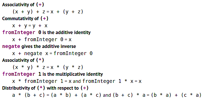 Fundamental laws of arithetic according to Num
What is this? Why is this mentioned? A simple starter explanation is
that we have here a set of guidelines for how addition and
multiplication must behave in order to have an instance of
Num. Let’s continue…
So if multiplication is just a glorified sort of addition, and division is glorified subtraction44 Multiplication is often phrased, e.g., “five fives,” i.e., five sets of five are to be considered (read added) together. Likewise, division "divide \(8\) by \(2\) is just subtract \(2\) from \(8\) over and over and keep track of how many times you can do this until there’s either nothing left or a number less than \(2\;\). , then that makes addition and subtraction the basis of arithmetic, but they have a very fundamentally different behavior when used in the wild that we must, in turn, account for. Yes, addition puts things together and subtraction takes something away from another thing. But there’s further -ness to addition that subtraction doesn’t have, namely, order doesn’t seem to matter, whereas it does with subtraction (and of course division). Obviously it matters which number gets subtracted or divided by which, but not with addition and multiplication.
We mentioned binary operators before, which means whenever we add or
subtract we’re really taking just two numbers at a time45
Think about it, even when you’ve got a whole list (vertical or
horizontal) of numbers to add, you’re really doing them two at a
time. One number becomes the addend and the other becomes the
augend, which is sort of a carrying-over holder to which the next
addend is added. So if we’re adding \(1 + 2 + 5\;\) we might add \(1 + 2\;\)
and then remember the augend is \(3\;\), then take addend \(5\) and add it
to augend \(3\) to get \(8\;\).
, i.e.,
the arity of the (+) operator is two, or (+) is a binary
operation. But again, why are we concerned with this?
Notice at GHC.Num it says
The Haskell Report defines no laws for
Num. However, (+) and (*) are customarily expected to define a ring and …
The Haskell Report is a reference manual for how Haskell is put
together, often just showing us how certain pieces of the language are
coded under the hood. Typically, you see a Backus-Naur
description46
More on Backus–Naur Form later. It’s used extensively to
create a metasyntax for programming languages. Maybe rabbit-hole this
Wikipedia treatment.
, then some description/talk, maybe also examples
and “translations47
Try Haskell’s list comprehension. Don’t expect to understand
what they’re saying just yet, but appreciate the magic and all the
devilish details. And while you’re at it you might further appreciate
just what a list comprehension is by looking at this Rosetta Code
article. Again, YMMV on what you can grasp at this point, but maybe
notice how Haskell is very Set-builder notation-friendly, while
other languages just seem to be kludging something together. Again,
maybe a bit too advanced, but check out Haskell’s entry for the
Pythagorean triplets. Experiment with the code. A big part of learning
to program is to read and experiment with code.
.” GHC.Num says there is no particular
mention in the HR of these arithmetical laws, but (+) and (*)
should define a ring. So here the lore is getting deep. What is
meant by a ring48
Have a look at this LibreText explanation but don’t try it
without first getting through the basic set theory stuff in the
assigned rabbit-hole.
? Well, a ring is something from abstract
algebra, which you’ll see in a mathematics curriculum once you’re
beyond Frosh college math including calculus, differential equations,
and linear algebra. The basic idea is that a ring is a set
containing a set of numbers, along with key arithmetical operators
behaving in certain ways. In other words, a ring is a sort of like a
package which includes numbers and the operations that work on those
numbers49
Algebra in higher math is redefined to be a system that always
“packages” a set of numbers with a set of useful operators/operations
on those numbers. It’s good to start thinking this way in order to
understand what Haskell and lots of computer science is doing and
saying.
. Then neatly bundled like this, we can do and say things about
them as a whole. But let’s leave it at that for now. We’ll soon
explore other similar “packagings” (semigroups, monoids, etc.) from
abstract algebra that are brought over for use in Haskell.
Continuing, if the so-called fundamental laws of arithmetic50 …taken from Richard Courant’s seminal What is Mathematics? say
- \(a + b = b + a\quad\) (additive commutativity, AC)
- \(ab = bc\quad\) (multiplicative commutativity, MC)
- \(a + (b + c) = (a + b) + c\quad\) (additive associativity, AA)
- \(a(bc) = (ab)c\quad\) (multiplicative associativity, MA)
- \(a(b + c) = ab + ac\quad\) (distributive law, DL)
then in order to have “number-ness” a Num instance for a number type
should have these behaviors when added or multiplied. But if we
compare, these five laws concerning addition and multiplication
aren’t exactly the same as those Haskell laws mentioned above from
GHC.Num. For one, Where’s #2, multiplicative commutativity, i.e., \(ab
= bc\;\)? It turns out not everything has MC; hence, we don’t want to
be obligated to defining MC for everything. An example is when
multiplying matrices. Maybe we’re not that far, but no, matrix
multiplication does not guarantee \(ab = bc\;\). Another potential
divergence is additive inverse and multiplicative inverse. These
should be defined on any type wanting to join the Num class. More on
that later.
\(\mathfrak{Fazit}\;\): Num is a super-class that is a prerequisite
“constraint” for anything number-like in Haskell. And so any type with
which we want to do basic arithmetic, i.e., to have number-ness, must
register an instance with the type class Num, defining the minimum
set of methods in order to perform basic math operations.
This has been a brief, hurried introduction to ordinality — with a small detour to explore some of the LE of what numbers are vis-à-vis Haskell and computers. The notion of order is everywhere and cannot be taken for granted. And the idea of ordinality goes pretty deep in higher math. See this and this fire hose treatments as somewhere between RO and RFYI. (And see this for something we’ll eventually take a Haskell stab at.) Note especially the order axioms and the properties of ordered fields. In general, these treatments are upper-level/grad math — or, yes, upper-level comp-sci, depending on your future school’s program. Remember, comp-sci dips and weaves around and through higher math with little or no warning — a bit like physics routinely takes off into high math-land as well.